Scaling Transformer Energy-Based Models for High Quality Image Synthesis

1MIT, 2UIUC, 3Harvard University
TL;DR We scale contrastively trained energy-based models to high-resolution ImageNet with a transformer energy function, reaching FID 3.82 (256×256) and 8.24 (512×512) without guidance, while keeping EBMs' special properties: composition, inpainting, OOD detection, and inference-time scaling.
512x512 sample 512x512 sample sample sample sample sample sample sample sample sample sample sample
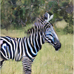
zebra
"zebra"
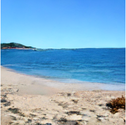
beach
"beach"
 $E_1 + E_2$
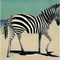
zebra + beach
composed result

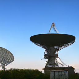
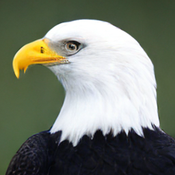
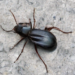
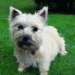
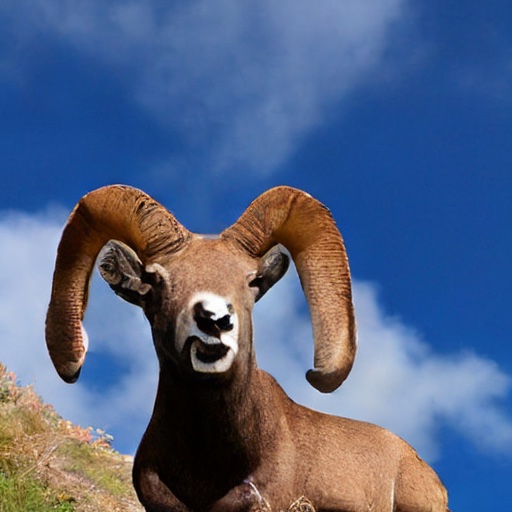
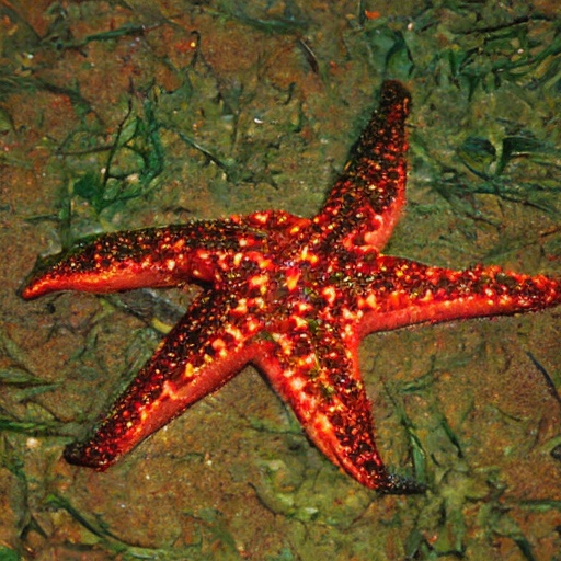
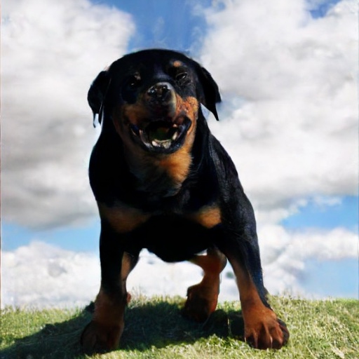
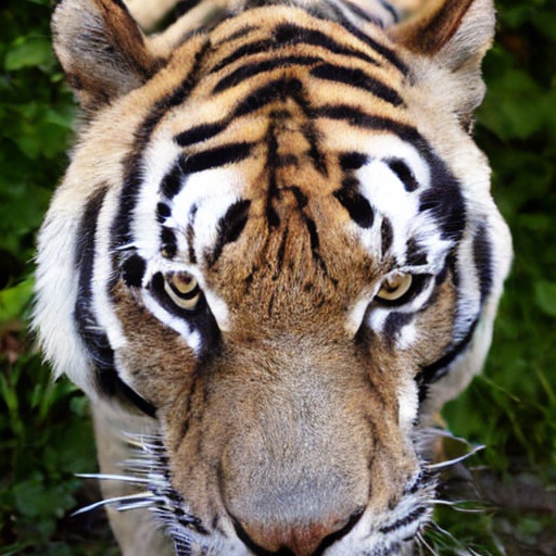
Left: uncurated class-conditional samples from TEM-XL/2 (80 sampling steps). The two large images are 512×512; the rest are 256×256. Right: summing the energy functions of two independent classes produces a coherent scene that satisfies both concepts, with no retraining.

Abstractclick to expand

Energy-Based Models (EBMs) are a flexible class of generative models that decouple probabilistic modeling from the generation process. This decoupling directly enables compositional generation and inference-time scaling, where sample quality can be refined simply by increasing sampling steps. However, severe challenges in high-dimensional sampling and training instabilities with deep architectures have restricted EBMs to low-dimensional regimes.

To resolve these bottlenecks, we introduce the Transformer Energy-Based Model (TEM), a scalable transformer energy function operating entirely within a latent space. On top of this backbone, we extract energies at multiple layers and sum them, composing complementary constraints from local texture to global semantics. Furthermore, two components make this high-quality at scale: Positive Representation Alignment (PRA), which supervises TEM's intermediate representations with a vision foundation model, and advanced sampling strategies that improve sample quality at inference.

TEM-XL achieves an FID-50K of 3.82 on class-conditional ImageNet 256×256 without classifier-free guidance, showing that a contrastive EBM can generate high-fidelity images. On ImageNet 512×512, TEM achieves an FID-50K of 8.24, demonstrating that the approach scales to higher resolution. We further validate the core promises of EBMs: compositional generation, zero-shot inpainting, and out-of-distribution detection.
How TEM trains and samples. During training, MCMC samples $x^-$ are drawn with Langevin dynamics and the energy is pushed down on real data $x^+$ and up on $x^-$. At inference, Langevin sampling on the trained energy descends the landscape and lands on the real data.

Scaling Behavior

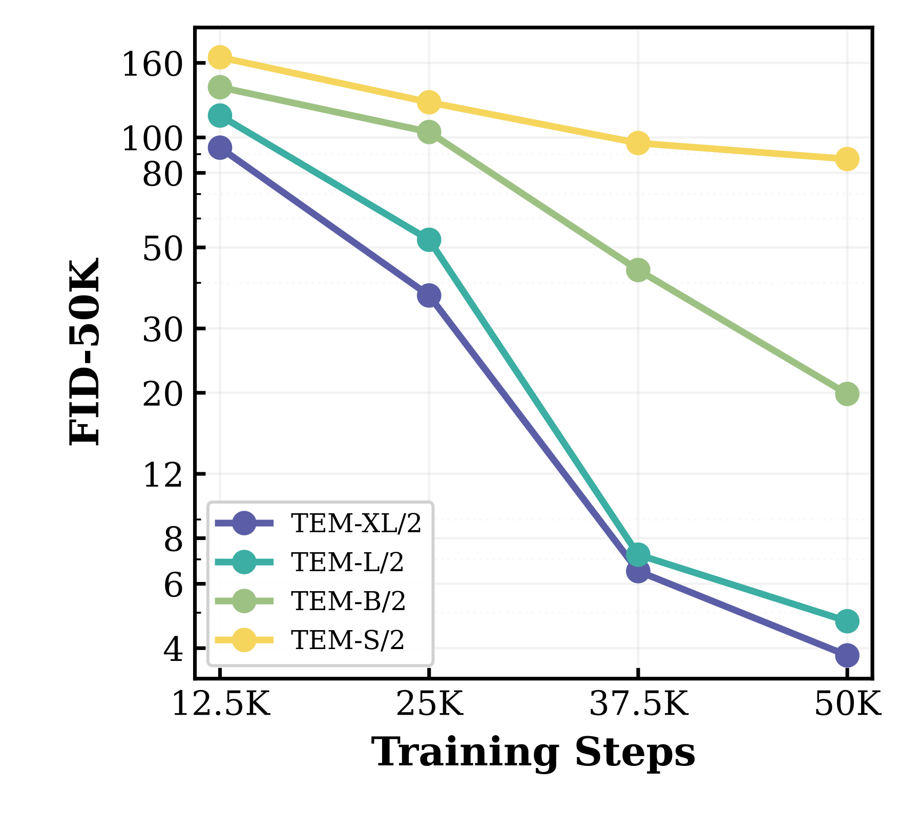
FID vs training steps FID vs training GFLOPs FID vs GFLOPs against diffusion baselines

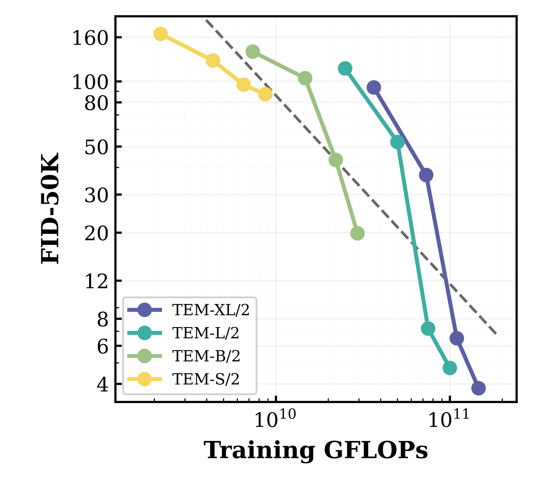
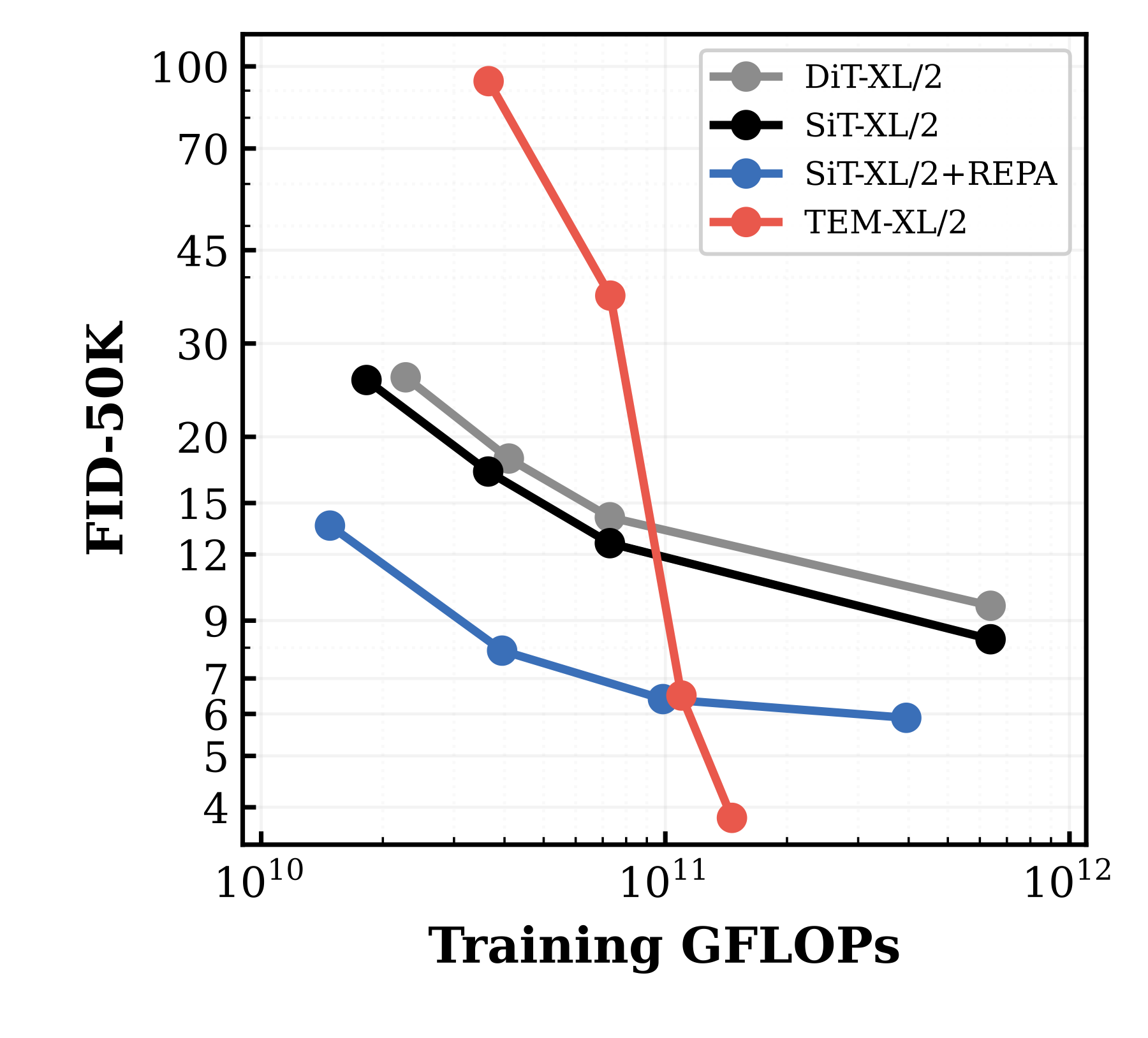
Left: FID-50K vs. training steps across model sizes; larger models are better at every checkpoint. Middle: all four sizes follow a consistent compute–quality trend. Right: TEM-XL against DiT-XL, SiT-XL and SiT-XL+REPA: TEM scales more steeply and reaches a lower unguided FID with less training compute.

Inference-Time Scaling

↔ Drag a slider below to step through sampling, from pure noise to the final sample.

Langevin sampling from pure noise ($T=0$) to $T=120$. Energy decreases steadily; at the training horizon (40 steps) coarse structure is established but residual noise remains, and continuing past it produces increasingly sharp, class-typical images.

Starting from another class’s image

↔ Drag a slider: the chain starts from an image of A and moves on B’s energy landscape only.

Each chain starts from an image of the source class (step 0) and runs 80 Langevin steps following only the target class’s energy gradient. The source energy (dashed) is never optimized, only measured: it rises purely as a side effect as the image leaves the source basin and settles into the target one.

Compositional Generation

+
pure Gaussian noise (sampling start) ?
composed result
energy image space → both concepts

Composition is just addition: the summed energy is lowest where both concepts are satisfied, so sampling on $E_1 + E_2$ lands on an image containing both.

For two energy-defined distributions, the product $p_1(x)p_2(x) \propto \exp(-(E_1(x)+E_2(x)))$. Sampling with the summed energy gives images that satisfy both concepts at once.

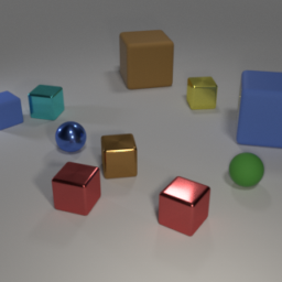
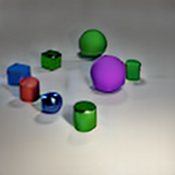
1 object
2 objects
3 objects
Datasetyellow = object location
CLEVR scene, 1 conditioned position
CLEVR scene, 2 conditioned positions
CLEVR scene, 3 conditioned positions
Generatedgreen = condition
TEM-B sample for 1 conditioned position
TEM-B sample for 2 conditioned positions
TEM-B sample for 3 conditioned positions
Model1 object2 objects3 objects
Comp. Diffusion0.8630.5980.262
TEM (ours)0.9560.7660.274

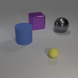
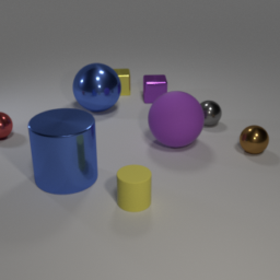
CLEVR 256×256 compositional generation. Top row: example dataset images; yellow boxes mark where objects are located. Bottom row: TEM-B samples conditioned on those locations; green boxes show the conditioned locations. Table: object detection success rate (↑) over 1,000 scenes, compared with Composable Diffusion.


Out-of-Distribution Detection

An EBM scores inputs directly: in-distribution data sits in the low-energy basin, while unfamiliar inputs land at high energy. A single forward pass of the unconditional energy $E_\theta(x)$ gives an OOD score, with no task-specific training, labels, or calibration. Diffusion baselines are scored by their denoising residual with one network evaluation. SiT+REPA receives the same DINOv2 alignment yet scores close to SiT, so alignment alone does not explain the gap: the scalar energy does.


In-distribution (ImageNet) E = 0.03 in-distribution · low E = 0.17 out-of-distribution · high
AUROC↑DiTSiTSiT-REPATEM
iNaturalist0.7770.7330.7800.904
Textures0.4390.4260.4380.687
Places3650.6690.6210.4810.636
SUN0.5050.5130.5000.640
Average0.5980.5730.5490.717

Left: a sample inside the in-distribution region gets low energy ($E = 0.03$), while a sample just outside it is flagged as out-of-distribution with high energy ($E = 0.17$); the OOD score is simply $S(x) = -E_\theta(x)$. Right: AUROC (↑) on four OOD benchmarks with ImageNet-1k validation as the in-distribution set.

Zero-Shot Inpainting

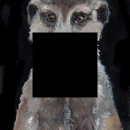
masked
Masked
T=0
$T=0$
T=20
$T=20$
T=40
$T=40$
T=60
$T=60$
T=80
$T=80$
masked
Masked
T=0
$T=0$
T=20
$T=20$
T=40
$T=40$
T=60
$T=60$
T=80
$T=80$

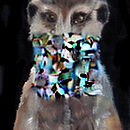
With an energy-based model, inpainting needs no retraining. We start sampling directly on the masked area, following the energy gradient only there while the rest of the image stays fixed, so the missing part fills in to match its surroundings.

Method

Multi-layer Energy Composition

TEM architecture
final head sample
$E_{\text{fin}}$: semantics
middle head sample
$E_{\text{mid}}$: layout
early head sample
$E_{\text{early}}$: texture
$\sum$
sample from summed energy
$E_{\text{early}} + E_{\text{mid}} + E_{\text{fin}}$

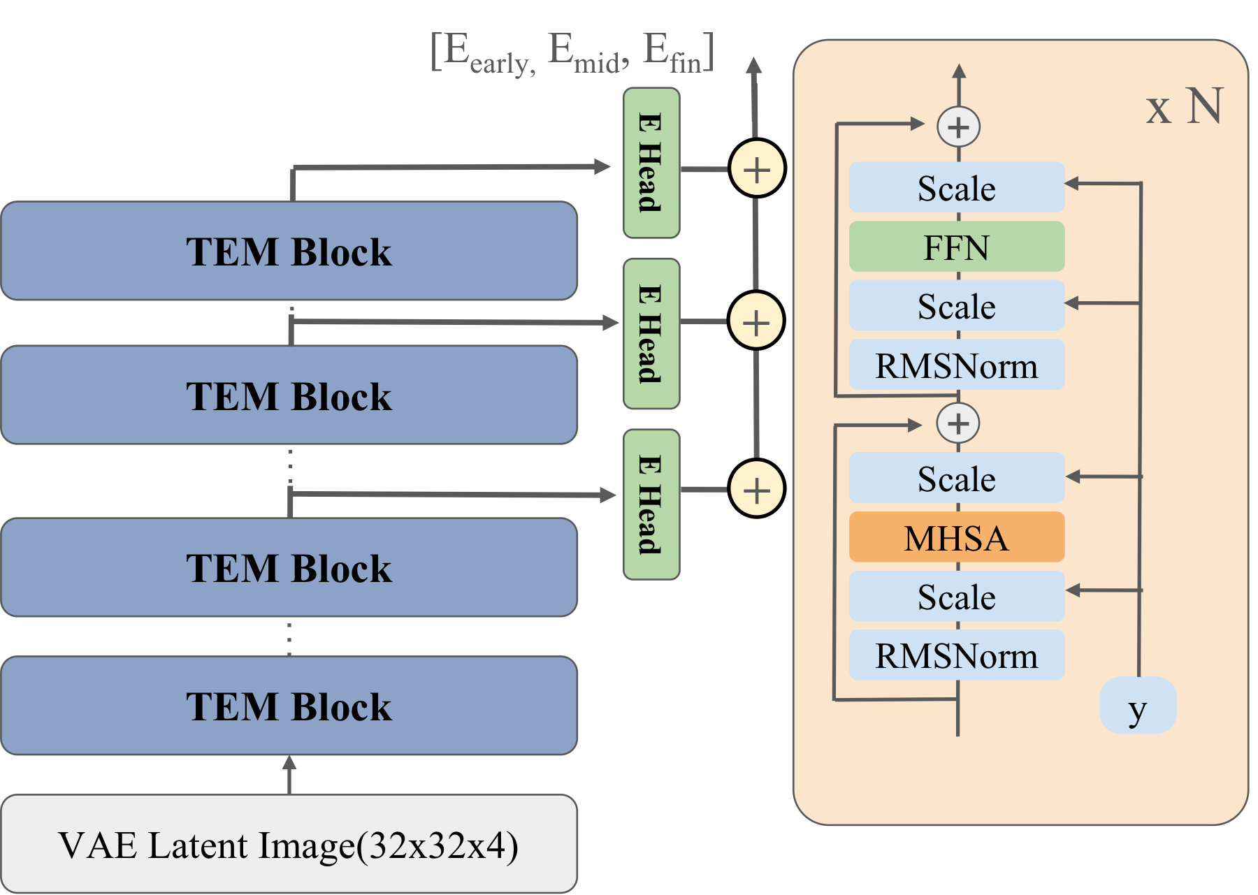
Multi-layer energy composition. TEM processes VAE-encoded latent tokens through a stack of TEM blocks, and energy heads at early, middle and final depths each output a scalar energy. Sampling from one head at a time shows what each one enforces: the early head recovers local texture without global structure, the middle head captures object layout without fine detail, and the final head keeps only coarse semantics. Sampling from their sum satisfies all three at once.

Positive Representation Alignment

02040608010012014016012.5K25K37.5K50KTraining stepsFID-50K ↓Without RA · 12.5K steps: FID 151.2Without RA · 25K steps: FID 107.5Without RA · 37.5K steps: FID 78.5Without RA · 50K steps: FID 42.842.8Pos+Neg RA · 12.5K steps: FID 155.6Pos+Neg RA · 25K steps: FID 107.4Pos+Neg RA · 37.5K steps: FID 63.2Pos+Neg RA · 50K steps: FID 36.636.6With PRA · 12.5K steps: FID 137.3With PRA · 25K steps: FID 103.5With PRA · 37.5K steps: FID 43.4With PRA · 50K steps: FID 19.919.9Without RAPos+Neg RAWith PRA
Positive phasedataset image x⁺ x⁺ (dataset) TEM E energy ↓ mid-layer features same x⁺Frozen VFM(DINOv2) ✓ align on the same clean x⁺ no alignment Negative phaseLangevin samples x⁻ x⁻ (Langevin) TEM E energy ↑ mid-layer features same x⁻ Frozen VFM(DINOv2) also aligned (Pos+Neg RA) no alignment (off-manifold) no alignment Intuition: only clean data at the bottom of the energy basin is aligned Pos+Neg RA: Langevin samples on the slopes are aligned too Without RA: nothing is aligned to the VFM energy ✓ x⁺ aligned dataset image (clean) ✗ x⁻: no alignment ✓ x⁻ aligned too

Left: FID-50K over training for TEM-B; the buttons step through the three settings and update the TEM diagram. PRA lowers FID from 42.8 to 19.9 at 50K steps, while also aligning negatives (Pos+Neg RA) reaches only 36.6. Right: switch between TEM and diffusion. Both align mid-layer features with a frozen VFM. Diffusion (REPA) aligns features of a noisy $x_t$ to the clean $x_0$ target, guiding denoising. TEM aligns only dataset images $x^+$, where both networks see the same clean input; Langevin samples $x^-$ get no alignment, since they lie off the data manifold and aligning them would work against the contrastive push.

More Samples

More on Energy-Based Models

Explore other work on energy-based models for generation, composition, and reasoning. More EBM works

BibTeX

@article{lee2026scaling,
  title         = {Scaling Transformer Energy-Based Models for High Quality Image Synthesis},
  author        = {Lee, Jungsoo and Gladstone, Alexi and Du, Yilun},
  journal       = {arXiv preprint arXiv:2610.31889},
  year          = {2026},
}